Hi,
I’ve used Code Saturne 2.0.7 for a couple of years to estimate pressure losses in hydraulic valves with generally good results. I’ve always used “mixing lenght” turbulence model for the good correspondence with experimental results and time of execution.
During the last week I tried to switch to Code Saturne 4 and I performed some comparisons. In particular, with the same mesh (about 280k tetra-elements), I compared the results of:
saturne 2.0.7 with mixing length
saturne 4 with mixing length
saturne 4 with k-eps
and I found very different results: there is about a factor of 3 in the estimation of the Delta P at the ports of the valve.
I used to make runs of about 800-1000 steps with steady state flow, increasing inlet flow rate every 100 steps.
I’ve attached:
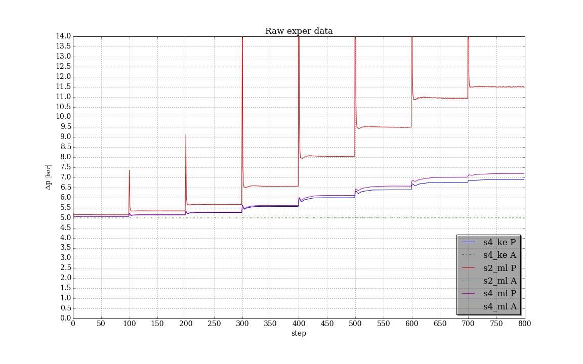
a graph plotting the pressure read at inlet (P port) and outlet (A port, fixed @5bar). Raw data are in Pascal, but have been scaled in the graph to bar
the 2 input files (I tried to keep the same parameters…)
I’ve also seen that, even if the pressure field is much smoother in saturne 4, when I import data in Paraview (Salome) the streamlines of fluid are much better distributed in saturne 2 (in sat 4 seem to stop somewhere… )
Thank you Yvan for your answer.
Here I’ve attached the listing files of the 3 simulations.
Now I’m running the same experiment with Saturne 2 and K-epsilon turbulence model.
I’ll post the results as soon as it finishes.
Then I’ll try your other suggestions.
Looking briefly at your v2 and v4 k-epsilon files, I saw that in 2.0, you do not use the same steady algorithm (idtvar -1/SIMPLE instead of idtvar 2/SIMPLEC).
Also, the initial density and laminar viscosity are the same, bu not the turbulent viscosity, probably due to ALMAX being set in 4.0 but not in 2.0. This can explain pretty big differences, though I am not sure it explains the whole difference (but it does make the computations difficult to compare from then).
Did you try IPHYDR (improved stratified velocity pressure) yet ?
Ccaccia73
Hello. I’m also interested in Code_Saturne and reliability of results obtained with it (for industrial applications). IMHO, calculating the local pressure drop is not so simple as it seems to be. Even commercial solvers may give some different results, although setup looks normal for this kind of tasks (fine mesh, prism layers of mesh cells near walls, SST turbulence, second order spatial discretisation).
Maybe calculation on refined mesh (for example, 1 million of cells) or other turbulence models (SST, RSM) will give results more close to experiment. Pressure loss in a valve is only local so it may be useful to look at particular flow features like recirculation zones and estimate mesh fineness in these areas.
Yvan
I’ve just finished the simulation with IPHYDR and there is no difference between those and the previous ones with same conditions (k-eps and Sat 4) at least in terms of pressure at inlet and outlet. I can post more detailed information if you need. btw it took me almost ‘forever’ (about 40 hours) to come to an end, while other simulations were much faster. I’m trying to investigate if working conditions were the same.
Antech
Happy to hear from you and maybe exchange opinions. I must say that I have little experience in the field: no particular training nor great budget, just a couple of years of trial and error… For my constraints (hardware and time) 1million cells is not feasible. My company produces hydraulic valves and their main interest is to have some tools that can predict flow-pressure drop relation for proportional valves: which generally means a lot of meshes (different connection, different opening…) and so a lot of simulations. I found a good compromise for the above constraints with Saturne 2: i.e. experimental data are close enough to the simulations for my purposes. Now I’m trying to see if I can replicate this with Saturne 4, mainly because I’m interested in some new features.
IPHYDR is slower because it requires additional pressure correction steps, but it was safe to check at least once that it does not influence the results…
Did you check the difference in hydraulic diameter (ALMAX) and time scheme ?
In any case, it is better to move to version 4.0, as 2.0 is not maintained anymore, so it is useful to understand why there is a difference.
If you have a smalll mesh (such as a subset of your geometry, with just the near-valve area, and possibly less refined), it could be interesting to check the differences on that one, as checks/comparisons could be run much more quicky (the smaller the mesh, the better, as long as the issue can be reproduced).
Thank you Yvan.
In my experience, working with a subset of the mesh (only the near-valve area) leads to difficult convergence, in particular because outlet conditions are not met.
I can definitely work with a slightly coarser mesh and/or the simplest possible geometry, at least for comparison.
In the next few days I’ll start checking ALMAX and time scheme for the current mesh.
Ccaccia73
OK, I see. So many variants is a problem with limited resources like PC (workstation). We usually solve less variants but with finer mesh and, in some cases, with specific physics.
About turbulence modeling. I’ve read a description of Mixing length and it seems to be the most simple zero-equation model that requires setting of characteristic length corresponding to specific geometry. I’m not a Saturne developer and cannot say what is the reason for difference in various versions with the same models, but I’d prefere SST for this kind of task with prism layers near walls at least for test (to chek if results will correspond to experiment), or, as basic setup, k-epsilon model (with relatively coarse mesh at the wall). Near-wall layers (for SST) are not very “cell-consuming”, but they should be added correctly to provide Y+ values for the first layer small enough (about 1.0) in the regions of interest (where the flow may separate).
Another detail is a turbulence characteristics at the inlet (for example, k and epsilon) that may affect the flow downstream significant in real cases. Saturne is smart enough to set them for us (in first approximation) provided we input a hydraulic diameter at the inlet (4*Area/Perimeter). With the zero-equation model (mixing length) you don’t need inlet turbulence parameters, but, IMHO, there is no guarantee that this simple model will give precise results.
Thank you Antech for the ideas you shared.
I’m planning to make more tests on the basis of your suggestions, when I have enough machine-time. I must also learn how to make good meshes.
Yvan, I made a new experiment, changing the Velocity-Pressure algorithm, from SIMPLEC to SIMPLE and it looks like it is the main responsible for the differences. Even if I wouldn’t say that the results converged to a steady state solution, they are much close to the ones obtained with sat2.
Ccaccia73
Some words about meshes for SST. I created them in Mesh module of Salome with NetGen (there are couple of NetGens, we need particular one). I used additional hypothesis in “3D” tab to introduce layers and played with them to obtain required Y+ (less than 1.0) but also to provide enough layers in turbulent part of boundary layer (it’s a small case, [300…500]*10^3 cells, so it runs fast on a PC). IMHO, Line Plot in ParaVis (ParaView) of tangential velocity in near-wall region is a good tool for estimation of boundary layer modelling quality (because it’s easy to distinguish “linear” and “logarythmic” parts). And, of course, a surface plot of Y+.
SIMPLEC to SIMPLE … looks like it is the main responsible for the differences
IMHO, it’s very strange. SIMPLE, SIMPLEC and PISO are velocity-pressure coupling methods and, as far as I know, they has nothing to deal with so large differencies of results (if we have a converged solutions). I hope I will check this on my test case.
I still need a very long time (about 16 hours) to finish the simulation
Please check the number of “linear” iterations (tables with rows starting with “c”). If you see more then 100 “linear” iterations for velocity then there may be a problem with mesh or timestep (if SIMPLEC is used). Would you please tell me what is the time per iteration (from Saturne’s output) and how many cells your current mesh consist of?
I perform tests on a usual PC (4 x 2600K cores) and it takes just about 30 minutes to obtain several hundrerds of iterations on ~500’000 cells mesh (Saturne 4.0.0).
Yvan Fournier
What may be the reason for this big difference between SIMPLE and SIMPLEC? I can’t get how does it possible for coupling sceme to affect the results in such extent… I’m interested in pressure drop calculations too so it’s important to me.
There should be no significant difference between the different SIMPLE, SIMPLEC and PISO algorithms, but there might be a slight sensitivity of the results to the time step du to the Rhie and Chow coupling (a disadvantage of colocated discretizations). Still, as the time step is local for steady methods, this is surprising, and the difference should be very minor.
Did you check the Courant/CFL values in the “listing” are close to 1 ? If not, the minimum or maximum time step value might be off.
Also, although it is important to converge computations for more precise results, the pressure drop itself usually varies only slightly, as it is often due mostly to the potential flow (established after the first iteration), then, often to a lesser degree, to the velocity and turbulence characteristics.
So it would be interesting to see how the pressure drop evolves over several iterations :
if it does not evolve much, you can run comparison tests with only a few iterations
if it evolves much, this would tend to indicate the turbulence model, or its parameters, are the major factor explaining the difference.
So in any case, checking this evolution of 20 or less time steps (and comparing to the results you have with many more iterations) can provide useful information.
SIMPLE, defaults.
Every case was allowed to calculate ~300 iterations. Then I compared pressure profiles in the slice just after inlet with ParaVis (ParaView) and found no sufficient difference. But there was no any large pressure difference (air) and flow pattern is different from valve. I plan to compose a dummy geometry more resembling the valve and repeat tests (if the reason will not be foubd here at that moment).
Update
Sorry, but I had no success with “valve test”. I still have Saturne only on my home PC (where there is no SolidWorks) and I can’t import “abstract valve” geometry in Salome (some bug in STEP reader). I did another calculation (for my work) on swirling nozzle geometry and calculated pressure drop was consistent (~20%) with simple formula (0.5Rhow^2). Settings was Steady + SIMPLE, Upwind for velocity, without flow reconstruction. Now I need to set exact initial data, perform more iterations and “precision run” with Centered scheme for velocity + flow reconstruction, but I don’t think that resulting pressure drop will differ significantly from simple estimation.
However nozzle case has geometry far different from valve, therefore I will now take an Internet survey on Salome STEP import bug…
Update 2
Hello. I worked with abstract valve geometry yesterday night. A saved this geometry in SolidWorks as STEP and played with STEP version, meters/millimeters and changing geometry. It didn’t help. Looks like a bug in Salome geometry import (though two other previous geometries imported correctly). So I used IGES + create shell + create solid, but I only had a time to build the mesh, then I switched to other case (needed to calculate a pressure drop on nozzle for my work). Hope I will get the valve test results soon (SIMPLE vs SIMPLEC).
Hallo,
sorry for the delay. I had a look at the listing files and saw that Courant number is way off (greater than 1 for SIMPLEC simulations).
So the next step will be to play with time step.
Are there any good practices to set minimal/maximal time step factor and maximal variation or should I just play with time step and let the defaults?
The number of linear iterations is much greater than 100 in each test.
I also tried to mesh as Antech suggested, but I’m finding difficulties, as the mesh is fairly complicated.
I think I’ll try to make some experience with a simpler geometry.
Ccaccia73 Courant number is way off (greater than 1)
AFAIK, for Saturne it may be up to 20 (50) without problems, although 1…5 is recommended.
The number of linear iterations is much greater than 100 in each test
Maybe it’s reasonable to switch to BiGCStab linear solver and set tolerance 10^-5 for all variables (even if you’ll reduce the time step). IMHO, it will not affect precision.
Sorry, cannot help you with mesh because your geometry is confidential (and my test case is on my home PC). But I foud it relatively simple to introduce prism layers provided you have marked groups (surfaces).
Ccaccia73 In my case there are small regions where Courant number is > 100
May be it’s a reason to use SIMPLEC with local timesteps. They are local spatially in Saturne, AFAIK.
I created a topic on Salome forum, there is an attach with “abstract” geometry outline. http://www.salome-platform.org/forum/forum_10/439129971
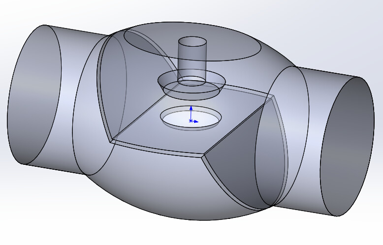
Geometry internals shown in attach to this message. Is this kind of geometry relevant? (I’m not working with valves, we use valves from another companies.)
Ccaccia73
Thanks for geometry. I see that it’s not a “classic” valve, looks more like a hydraulic switch, if I got it right… I understand that particular details are confidential so I will work with my “classic” abstract geometry. Hope that conclusion about SIMPLE/SIMPLEC sensitivity will be applicable also to your tasks.


